Transition States#
In addition to generating full reaction profiles directly autodE provides automated access to transition states (TSs). TSs are found either from a reaction, where bond rearrangements are found and TS located along each possible path, or from 3D structures of reactants & products, and a given bond rearrangement.
Warning
Transition states have no check that the stereochemistry is correctly preserved.
Default: Reaction#

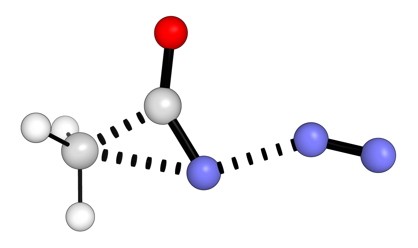
For a simple Curtius rearrangement copied as a SMILES string directly from ChemdrawTM (selecting reactants and products with arrows and ‘+’ then Edit->Copy As->SMILES) the TS can be located with
import autode as ade

ade.Config.n_cores = 8

rxn = ade.Reaction("CC(N=[N+]=[N-])=O>>CN=C=O.N#N")
rxn.locate_transition_state()
rxn.ts.print_xyz_file(filename="ts.xyz")
Out (visualised)
Note
locate_transition_state only locates a single transtion state for
each possible bond rearrangment and does not attempt to search the conformational
space.
CI-NEB#
Minimum energy pathways can also be generated using nudged elastic band (NEB) calculations. To find the peak species suitable as a TS guess geometry for the prototypical Claisen rearrangement ([3,3]-sigmatropic rearrangement of allyl phenyl ether)
import autode as ade

reac = ade.Reactant("claisen_r.xyz")
prod = ade.Product("claisen_p.xyz")

# Create an 8 image nudged elastic band with intermediate images interpolated
# from the final points, thus they must be structurally similar
neb = ade.CINEB.from_end_points(reac, prod, num=8)
# minimise with XTB
neb.calculate(method=ade.methods.XTB(), n_cores=4)

# print the geometry of the peak species
print("Found a peak: ", neb.images.contains_peak)
neb.peak_species.print_xyz_file(filename="peak.xyz")
Out:
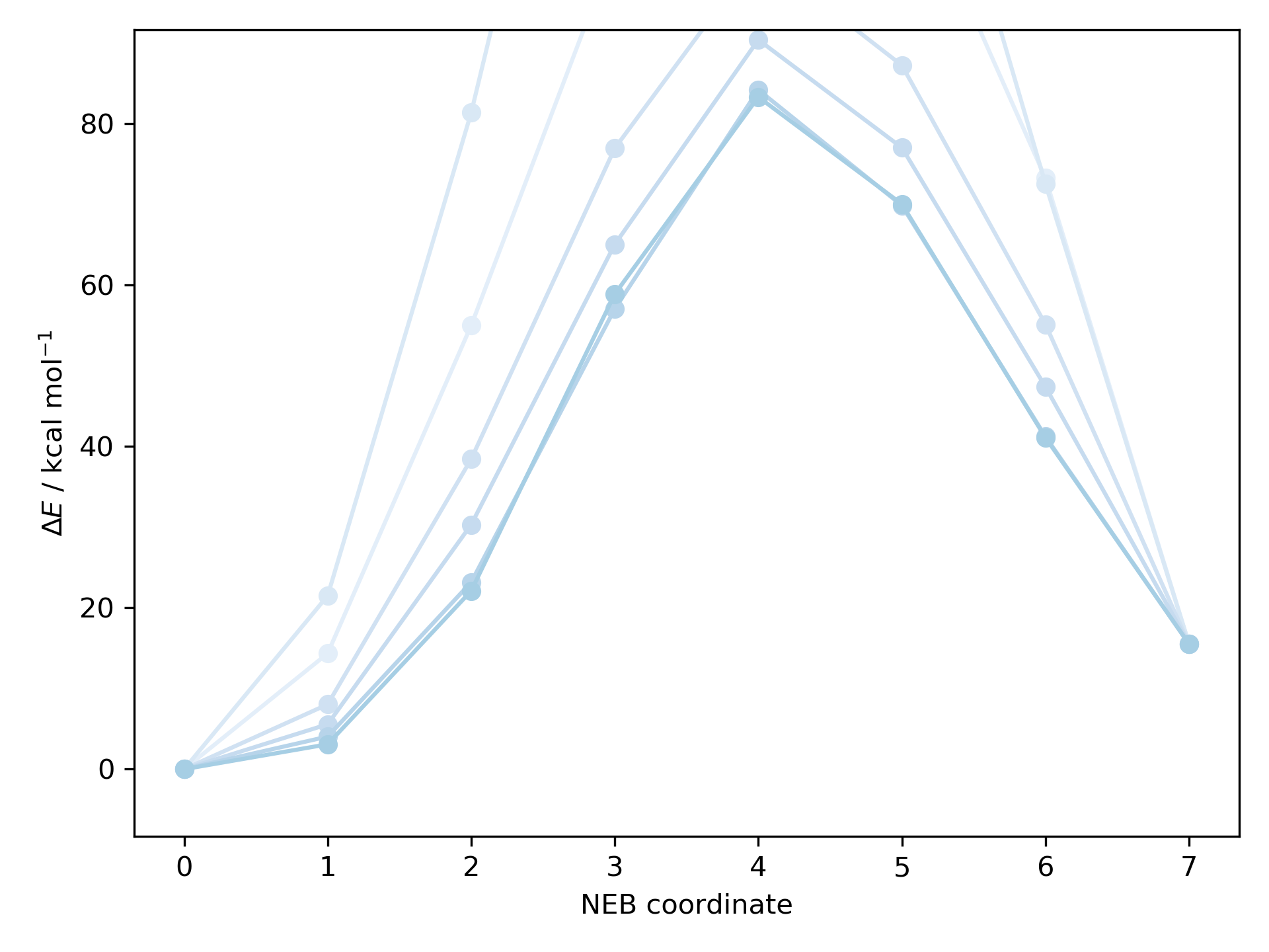
Out (visualised):
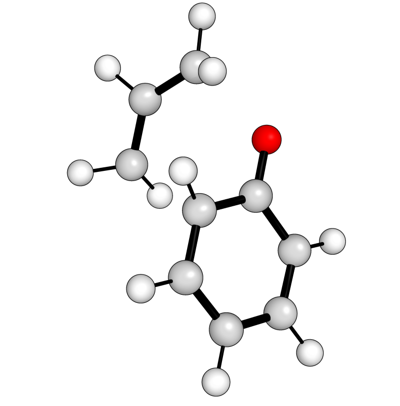
where the xyz files used are:
20
claisen_r
C  -3.98726   0.74520  0.45281
C  -4.50106  -0.55204  0.38563
C  -2.98263   1.15687 -0.42991
C  -2.51083   0.25840 -1.40799
C  -3.03021  -1.03906 -1.47415
C  -4.01895  -1.44546 -0.57369
O  -2.47596   2.40755 -0.27307
C  -1.33638   2.94073 -0.85085
H  -1.73709   0.54678 -2.10649
H  -2.65792  -1.73268 -2.21661
H  -4.41017  -2.45344 -0.61689
H  -4.35505   1.42777  1.20883
H  -5.26464  -0.86554  1.08531
C  -0.04683   2.27939 -0.39973
H  -1.28052   4.00673 -0.54623
H  -1.40915   2.91149 -1.95905
C   0.04395   1.20681  0.40079
H   0.87953   2.71662 -0.75770
H  -0.81785   0.69435  0.80686
H   1.01980   0.81060  0.65942
20
claisen_p
C   -4.34571   0.63520   0.57310
C   -4.49777  -0.68069   0.34490
C   -3.23250   1.40679   0.03037
C   -2.22119   0.64743  -0.81975
C   -2.49978  -0.80349  -0.98985
C   -3.56127  -1.41597  -0.45542
O   -3.11541   2.59776   0.24431
C   -0.59568   3.13650  -1.35460
H   -2.24578   1.10277  -1.81941
H   -1.78329  -1.35547  -1.58358
H   -3.73211  -2.47147  -0.60583
H   -5.04256   1.18717   1.18701
H   -5.33408  -1.21816   0.77022
C   -0.15430   2.17960  -0.56309
H   -0.03493   4.04448  -1.49486
H   -1.53872   3.08831  -1.87085
C   -0.79076   0.85415  -0.27213
H    0.79501   2.30610  -0.05582
H   -0.80710   0.70442   0.81159
H   -0.14130   0.07563  -0.68902
Note
NEBs initialised from end points use linear interpolation then an image independent pair potential to relax the initial linear path, following this paper.