1D PES Generation#
autodE allows for both potential energy surface (PES) to be constructed where other degrees of freedom are frozen (unrelaxed) or allowed to optimise (relaxed).
Unrelaxed#
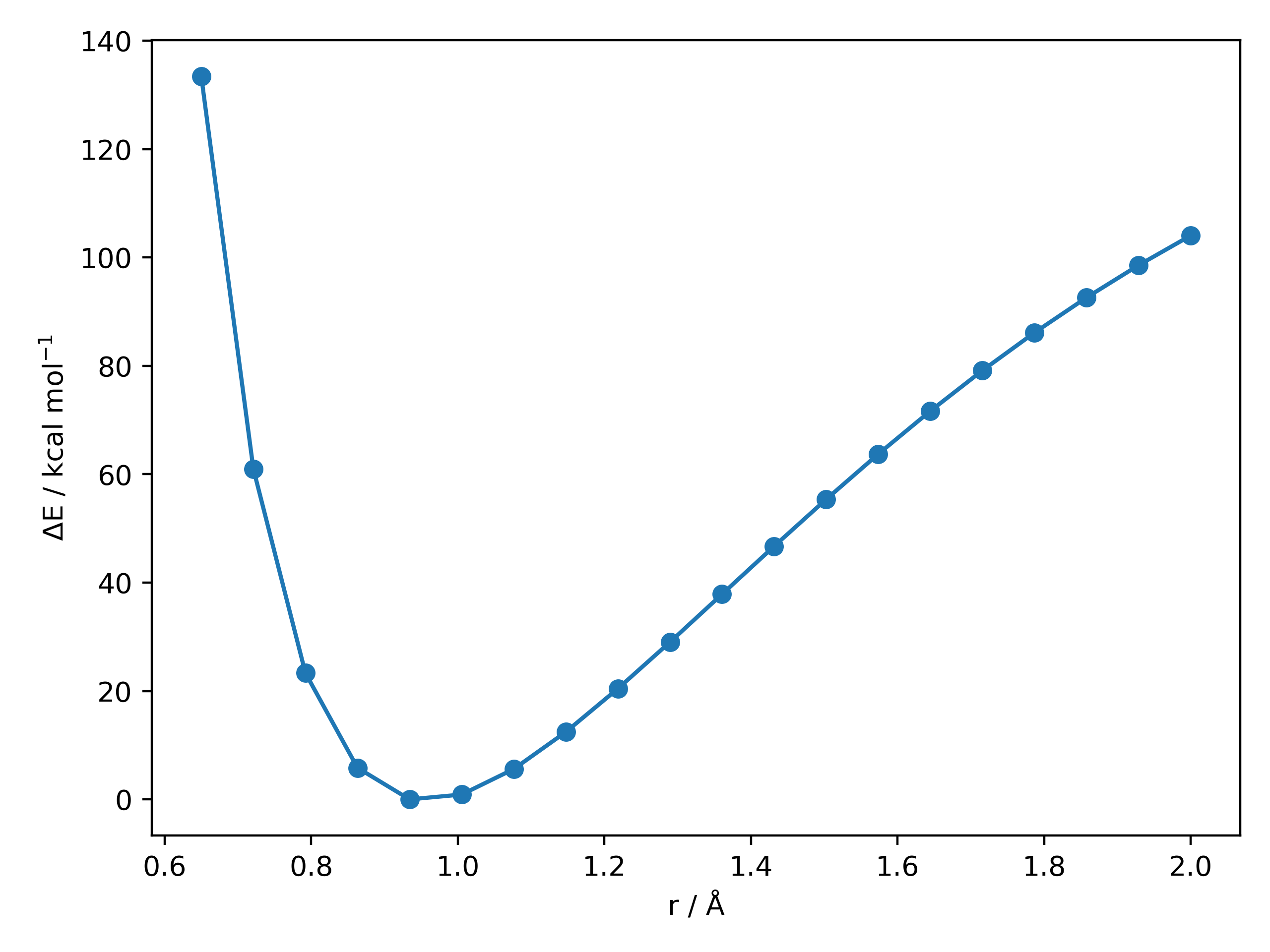
For the O-H dissociation curve in H2O at the XTB level:
import autode as ade
import matplotlib.pyplot as plt

water = ade.Molecule(name="H2O", smiles="O")
# water.atoms = [[O, x, y, z], [H, x', y', z'], [H, x'', y'', z'']]

# Initialise the unrelaxed potential energy surface over the
# O-H bond from 0.65 Å to 2.0 Å in 20 steps
pes = ade.pes.UnRelaxedPES1D(species=water, rs={(0, 1): (0.65, 2.0, 20)})

# Calculate the surface using the XTB tight-binding DFT method
pes.calculate(method=ade.methods.XTB())

# Finally, plot the surface using matplotlib
plt.plot(pes.r1, pes.relative_energies.to("kcal mol-1"), marker="o")

plt.ylabel("ΔE / kcal mol$^{-1}$")
plt.xlabel("r / Å")
plt.savefig("OH_PES_unrelaxed.png", dpi=400)
Out (OH_PES_unrelaxed.png):
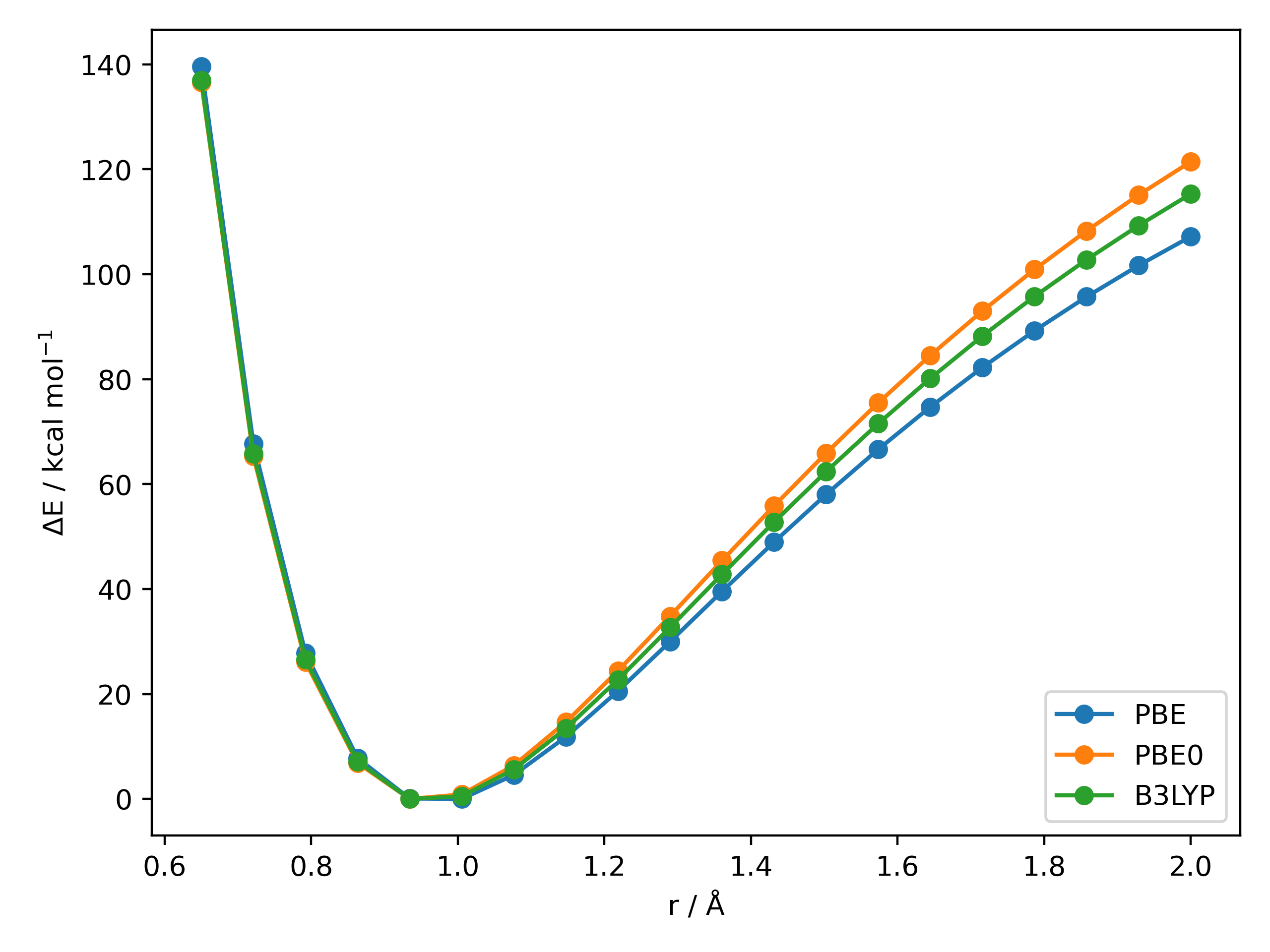
For the same O-H 1D PES scan using a selection of different DFT methods:
import autode as ade
import matplotlib.pyplot as plt

# Initialise the PES over the O-H bond 0.65 -> 2.0 Å
pes = ade.pes.UnRelaxedPES1D(
    species=ade.Molecule(name="H2O", smiles="O"), rs={(0, 1): (0.65, 2.0, 20)}
)

# For the three different DFT functionals calculate the PES and plot the line
for functional in ("PBE", "PBE0", "B3LYP"):
    pes.calculate(method=ade.methods.ORCA(), keywords=[functional, "def2-SVP"])

    plt.plot(
        pes.r1,
        pes.relative_energies.to("kcal mol-1"),
        marker="o",
        label=functional,
    )

# Add labels to the plot and save the figure
plt.ylabel("ΔE / kcal mol$^{-1}$")
plt.xlabel("r / Å")
plt.legend()
plt.tight_layout()
plt.savefig("OH_PES_unrelaxed_DFT.png", dpi=400)
Out (OH_PES_unrelaxed2.png):
Relaxed#
A relaxed 1D PES can be generated and plotted using the default plot
method for the same O-H stretch using:
import autode as ade

water = ade.Molecule(name="H2O", smiles="O")

# Initialise a relaxed potential energy surface for the water O-H stretch
# from 0.65 -> 2.0 Å in 15 steps
pes = ade.pes.RelaxedPESnD(species=water, rs={(0, 1): (0.65, 2.0, 15)})

pes.calculate(method=ade.methods.XTB())
pes.plot("OH_PES_relaxed.png")

# PESs can also be saved as compressed numpy objects and reloaded
pes.save("pes.npz")

# For example, reload the PES and print the distances and energies
pes = ade.pes.RelaxedPESnD.from_file("pes.npz")

print("r (Å)   E (Ha)")
for i in range(15):
    print(f"{pes.r1[i]:.4f}", f"{pes[i]:.5f}")
Out (OH_PES_relaxed.png):
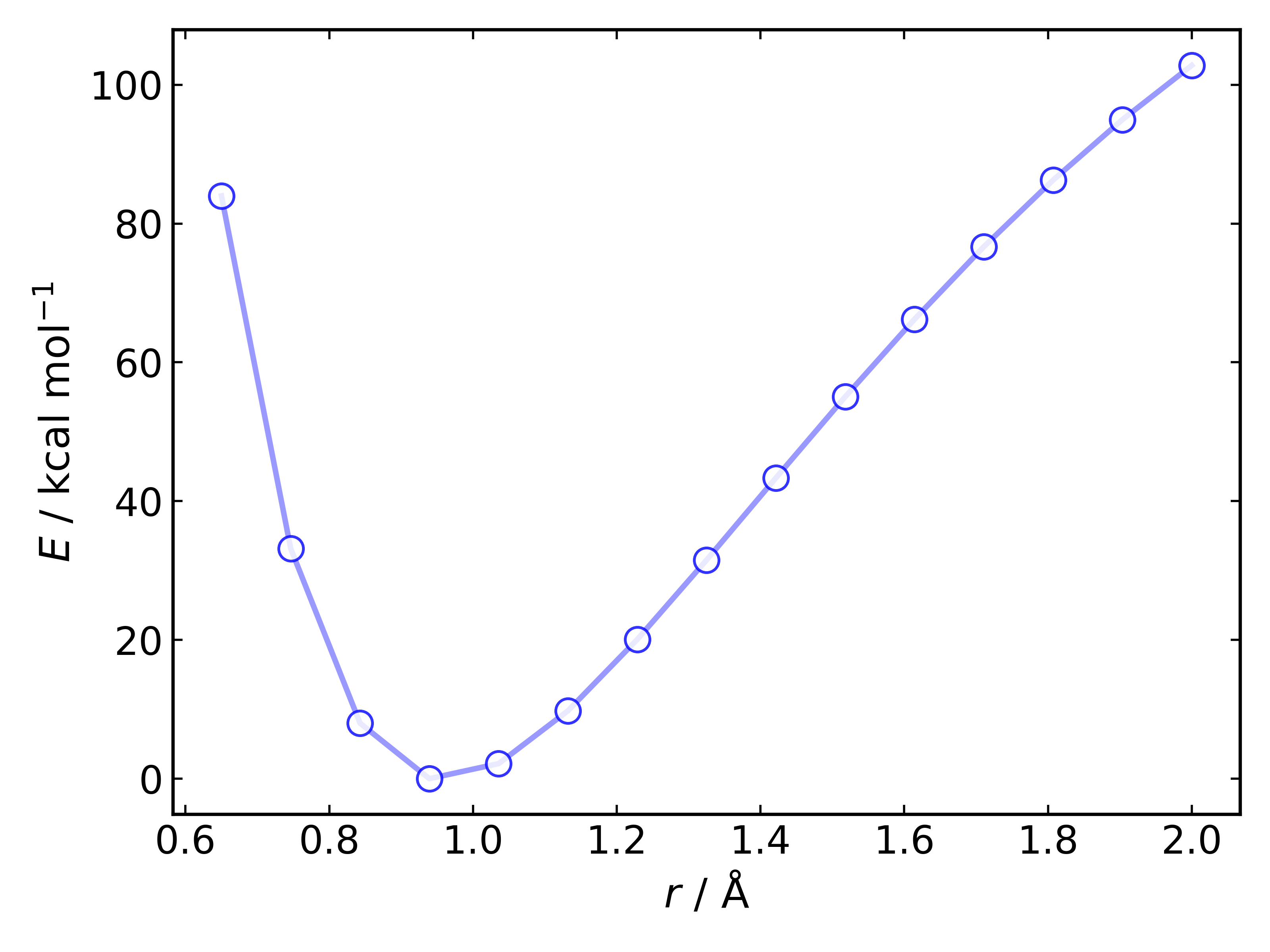
r_1 (Å)   E (Ha)
0.6500   -4.93638
0.7464   -5.01741
0.8429   -5.05749
0.9393   -5.07023
1.0357   -5.06677
1.1321   -5.05464
1.2286   -5.03825
1.3250   -5.02002
1.4214   -5.00116
1.5179   -4.98253
1.6143   -4.96472
1.7107   -4.94807
1.8071   -4.93276
1.9036   -4.91887
2.0000   -4.90642